Temporal-Difference Learning

TD learning is a combination of Monte Carlo ideas and dynamic programming (DP) ideas. Like Monte Carlo methods, TD methods can learn directly from raw experience without a model of the environment’s dynamics. Like DP, TD methods update estimates based in part on other learned estimates, without waiting for an outcome (they bootstrap).

TD Prediction

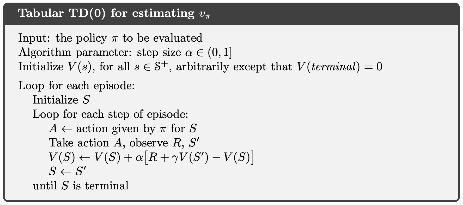
Whereas Monte Carlo methods must wait until the end of the episode to determine the increment to $V\left(S_t\right)$ (only then is $G_t$ known), TD methods need to wait only until the next time step. At time $t+1$ they immediately form a target and make a useful update using the observed reward $R_{t+1}$ and the estimate $V\left(S_{t+1}\right)$. The simplest TD method makes the update

$$V\left(S_t\right) \leftarrow V\left(S_t\right)+\alpha\left[R_{t+1}+\gamma V\left(S_{t+1}\right)-V\left(S_t\right)\right]$$

immediately on transition to $S_{t+1}$ and receiving $R_{t+1}$. In effect, the target for the Monte Carlo update is $G_t$, whereas the target for the TD update is $R_{t+1}+\gamma V\left(S_{t+1}\right)$. This TD method is called TD $(0)$, or one-step $T D$, because it is a special case of the $\operatorname{TD}(\lambda)$.

Finally, note that the quantity in brackets in the $\operatorname{TD}(0)$ update is a sort of error, measuring the difference between the estimated value of $S_t$ and the better estimate $R_{t+1}+\gamma V\left(S_{t+1}\right)$. This quantity, called the TD error, arises in various forms throughout reinforcement learning:

$$\delta_t \doteq R_{t+1}+\gamma V\left(S_{t+1}\right)-V\left(S_t\right)$$

Notice that the TD error at each time is the error in the estimate made at that time. Because the TD error depends on the next state and next reward, it is not actually available until one time-step later. That is, $\delta_t$ is the error in $V\left(S_t\right)$, available at time $t+1$. Also note that if the array $V$ does not change during the episode (as it does not in Monte Carlo methods), then the Monte Carlo error can be written as a sum of TD errors:

$$\begin{aligned} G_t-V\left(S_t\right) &=R_{t+1}+\gamma G_{t+1}-V\left(S_t\right)+\gamma V\left(S_{t+1}\right)-\gamma V\left(S_{t+1}\right) \\ &=\delta_t+\gamma\left(G_{t+1}-V\left(S_{t+1}\right)\right) \\ &=\delta_t+\gamma \delta_{t+1}+\gamma^2\left(G_{t+2}-V\left(S_{t+2}\right)\right) \\ &=\delta_t+\gamma \delta_{t+1}+\gamma^2 \delta_{t+2}+\cdots+\gamma^{T-t-1} \delta_{T-1}+\gamma^{T-t}\left(G_T-V\left(S_T\right)\right) \\ &=\delta_t+\gamma \delta_{t+1}+\gamma^2 \delta_{t+2}+\cdots+\gamma^{T-t-1} \delta_{T-1}+\gamma^{T-t}(0-0) \\ &=\sum_{k=t}^{T-1} \gamma^{k-t} \delta_k \end{aligned}$$

This identity is not exact if $V$ is updated during the episode (as it is in $\operatorname{TD}(0)$ ), but if the step size is small then it may still hold approximately. Generalizations of this identity play an important role in the theory and algorithms of temporal-difference learning.

Advantages of TD Prediction Methods

• TD methods generally converge faster than MC methods, although this has not been formally proven.
• TD methods do converge on the value function with a sufficiently small step size parameter, or with a decreasing step size.
• They are extremely useful for continuing tasks that cannot be broken down in episodes as required by MC methods.

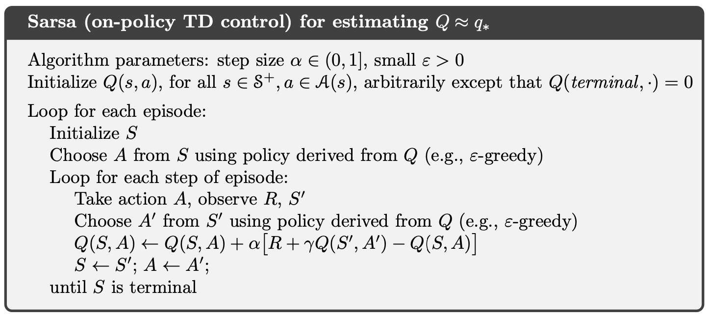
Sarsa: On-policy TD Control

In the previous section, we considered transitions from state to state and learned the values of states. Now we consider transitions from state-action pair to state-action pair and learn the values of state-action pairs. Formally these cases are identical: they are both Markov chains with a reward process. The theorems assuring the convergence of state values under $\operatorname{TD}(0)$ also apply to the corresponding algorithm for action values:

$$Q\left(S_t, A_t\right) \leftarrow Q\left(S_t, A_t\right)+\alpha\left[R_{t+1}+\gamma Q\left(S_{t+1}, A_{t+1}\right)-Q\left(S_t, A_t\right)\right]$$

This update is done after every transition from a nonterminal state $S_t$. If $S_{t+1}$ is terminal, then $Q\left(S_{t+1}, A_{t+1}\right)$ is defined as zero. This rule uses every element of the quintuple of events, $\left(S_t, A_t, R_{t+1}, S_{t+1}, A_{t+1}\right)$, that make up a transition from one state-action pair to the next. This quintuple gives rise to the name Sarsa for the algorithm.

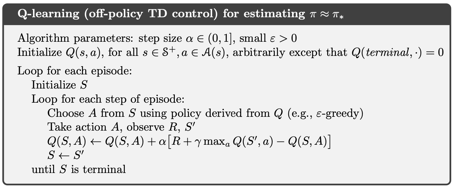
Q-learning: Off-policy TD Control

One of the early breakthroughs in reinforcement learning was the development of an off-policy TD control algorithm known as Q-learning (Watkins, 1989), defined by

$$Q\left(S_t, A_t\right) \leftarrow Q\left(S_t, A_t\right)+\alpha\left[R_{t+1}+\gamma \max _a Q\left(S_{t+1}, a\right)-Q\left(S_t, A_t\right)\right]$$

In this case, the learned action-value function, $Q$, directly approximates $q_*$, the optimal action-value function, independent of the policy being followed. This dramatically simplifies the analysis of the algorithm and enabled early convergence proofs. The policy still has an effect in that it determines which state-action pairs are visited and updated. However, all that is required for correct convergence is that all pairs continue to be updated.

Concurrent Q-Learning

• Check out Concurrent Q-Learning here.

Expected Sarsa

Instead of updating our value function with the value maximizing action at $S_{t+1}$ (as is the case with Q-learning) or with the action prescribes by our $\epsilon$-greedy policy (as is the case with SARSA), we could make updates based on the expected value of $Q$ at $S_{t+1}$. This is the premise of expected sarsa. Doing so reduces the variance induced by selecting random actions according to an $\epsilon$-greedy policy. Its update is described by:

$$\begin{aligned} Q\left(S_t, A_t\right) & \leftarrow Q\left(S_t, A_t\right)+\alpha\left[R_{t+1}+\gamma \mathbb{E}_\pi Q\left(S_{t+1}, A_{t+1} \mid S_{t+1}\right)-Q\left(S_t, A_t\right)\right] \\ & \leftarrow Q\left(S_t, A_t\right)+\alpha\left[R_{t+1}+\gamma \sum_a \pi\left(a \mid S_{t+1}\right) Q\left(S_{t+1}, a\right)-Q\left(S_t, A_t\right)\right] \end{aligned}$$

We can adapt expected SARSA to be off-policy by making our target policy $\pi$ greedy, in which case expected SARSA becomes Q-learning. It is therefore seen as a generalization of Q-learning that reliably improves over Sarsa.